Jekyll2026-06-05T12:19:23-07:00https://pipeparodi.com/feed.xmlFelipe ParodiComputational Neuroethologist | PhD Candidate at UPenn | Research in AI, Deep Learning, and Primate Behavior | Specializing in Social Interaction AnalysisFelipe ParodiAwesome Active Inference: a community resource2026-05-27T00:00:00-07:002026-05-27T00:00:00-07:00https://pipeparodi.com/blog/awesome-active-inference GitHub
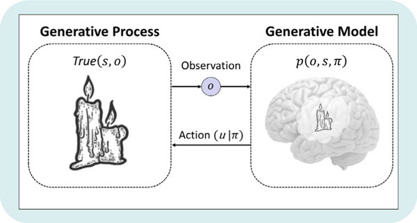
Active inference is the claim that perception, action, and learning are all one process. An agent perceives and acts so as to minimize surprise, the gap between what it senses and what its model of the world predicted. Over about two decades Karl Friston and others have stretched this one idea to cover the cortex, psychiatric symptoms, robot control, and reinforcement learning.
The whole setup in one picture. The world and the agent's model of it touch at only two points, what the agent observes and what it does. Everything in between is inference. From Smith, Friston & Whyte, J. Math. Psychol. 2022 (CC BY-NC-ND 4.0).
I think it is one of the most interesting ideas in neuroscience, and one of the hardest to actually learn. The papers run across twenty years and several fields that barely cite each other, the math is heavy, and most introductions assume you have already read the other introductions. I bounced off it a few times before it stuck. Awesome Active Inference is the reading list I wish someone had handed me at the start. It runs from textbooks and tutorials through the original free-energy papers, predictive coding, the discrete and continuous-time formulations, deep active inference, computational psychiatry, and the software libraries, in roughly the order I would read them now. There are two starting points at the top. Neuroscientists and machine-learning people need almost entirely different first papers, and the list says which.
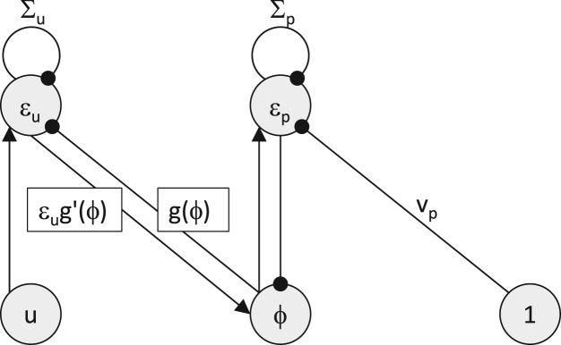
The fastest way in for me was predictive coding, the idea that the cortex spends most of its effort predicting its own inputs and passing the errors upward. Rafal Bogacz’s 2017 tutorial writes this out as a small circuit you can actually simulate.
Predictive coding as an actual circuit. Nodes send predictions down and prediction errors (ε) back up, using only local connections. From Bogacz, J. Math. Psychol. 2017 (CC BY 4.0).
The other half is decision-making. In the discrete-state version an agent plans over a POMDP and trades off getting reward against getting information. Exploration drops out of the same quantity the agent is already minimizing. The continuous-time version connects to control theory and robotics. The same machinery serves as both a theory of what brains do and a recipe for building agents.
A toy task from Smith et al.'s tutorial. Two slot machines, a hint you can pay for, and a choice about whether the information is worth the cost. This is what a POMDP looks like once it is concrete. From Smith, Friston & Whyte, J. Math. Psychol. 2022 (CC BY-NC-ND 4.0).
Like the Awesome Computational Primatology list, this is a public GitHub repo. If some paper, tutorial, lecture, or library is the thing that made active inference click for you, please add it.
]]>Felipe ParodiZero-Ablation Overstates Register Function in Vision Transformers2026-03-04T00:00:00-08:002026-03-04T00:00:00-08:00https://pipeparodi.com/blog/register-tokens-information-flow Code Paper PDF Cite
Jonas and Kording (2017) applied standard neuroscience analysis techniques to a microprocessor, lesioning individual transistors and measuring which were “necessary” for running Donkey Kong. The results were confident, publishable – and entirely misleading. Lesioning a component and observing what breaks reveals that the component was involved in the circuit, not that it computed the thing that broke.
We encountered an analogous problem with vision transformers.
Zero-ablation – replacing token activations with zero vectors – is (was?) a widely used tool for probing token function in ViTs. When we zeroed register tokens in DINOv2+registers and DINOv3, classification dropped 36.6 pp and segmentation dropped 30.9 pp. Registers appeared functionally indispensable. Yet when we replaced registers with dataset-mean activations, Gaussian noise, or even registers from completely different images, every task was preserved within 1 pp of baseline. The specific content of registers is dispensable; only their presence matters.
Registers do play a real structural role: they buffer dense features from CLS dependence (zeroing CLS collapses segmentation by 37 pp without registers but <1 pp with them), and they compress patch geometry (effective rank 13.5 → 4.0). Their per-image content, however, is interchangeable. Zero-ablation overstated the story because zero vectors are out-of-distribution – the network never encountered them during training, and injecting them cascades disruption through every subsequent layer.
The remainder of this post describes each experiment and its implications.
Background: ViTs, CLS, and Registers
A Vision Transformer (ViT) divides an image into non-overlapping patches (typically 14×14 pixels), converts each patch into a vector, and prepends a learnable CLS token. All tokens interact through self-attention across multiple layers, where each token can attend to every other token to aggregate information. At the output, CLS serves as a global image summary (used for classification), while patch tokens retain spatial information (used for segmentation and correspondence). This global–spatial distinction underlies the experiments below.
Figure 1. Our setup. A ViT processes an image as CLS + register + patch tokens. We replace CLS or register outputs with zeros, dataset means, noise, or cross-image shuffled values, then measure impact on global tasks (classification, retrieval) and dense tasks (correspondence, segmentation).
Patch features are rich and spatially structured. Below, they are projected into three PCA components (mapped to RGB):
Interactive: PCA patch features
Image:
The artifact problem and register tokens
Darcet et al. (2024) found that large self-supervised ViTs produce high-norm artifact tokens in low-information regions – patches over sky, water, or uniform backgrounds develop anomalously large activations that distort downstream feature maps. Their fix: append 4 learnable register tokens to the input. Registers participate in attention but are discarded at inference, absorbing the artifact computation and leaving patch tokens clean.
DINOv3 (Simeoni et al., 2025) builds on this with Gram anchoring – a training objective that encourages patches to preserve their pairwise spatial relationships. The combination of registers and Gram anchoring produces the current state-of-the-art for dense features. We set out to determine what functional role registers play in this configuration.
The norm heatmaps below illustrate the artifact problem: bright regions indicate high-norm patches. Compare DINOv2 (artifacts in uniform regions) with register-equipped models:
Interactive: Patch norm heatmaps
Image:
Zero-Ablation Results
We zeroed CLS or register tokens at every transformer layer and measured the downstream impact on four tasks:
Task
Type
Metric
What it measures
Classification
Global
Top-1 accuracy
Can a linear classifier read object identity from CLS?
kNN retrieval
Global
Recall@1
Can CLS find the most similar image?
Correspondence
Dense
Accuracy
Can patches match the same object part across images?
Segmentation
Dense
mIoU
Can patches assign correct semantic labels?
The interactive heatmap below summarizes the full ablation results. Toggle between raw accuracy and delta-from-baseline:
CLS zeroing: dense tasks are buffered
In DINOv2 (no registers), zeroing CLS is catastrophic across all tasks: classification drops from 73.2% to 0.1%, correspondence falls 15.9 pp, segmentation falls 37.1 pp.
With registers present, the pattern is markedly different. CLS zeroing still eliminates classification (the linear probe reads from CLS, so this is expected), but dense tasks are largely unaffected:
Registers have absorbed the role CLS previously played for spatial features. Patch representations no longer depend on CLS.
Register zeroing: everything collapses
Zeroing registers produces large drops, especially in DINOv3:
Classification: 62.0% → 25.4% (−36.6 pp)
Segmentation: 78.5% → 47.6% (−30.9 pp)
Correspondence: 78.9% → 57.8% (−21.1 pp)
Taken at face value, registers appear to carry critical information that the network depends on. This interpretation, however, does not hold up.
You can see the ablation effects directly in patch PCA features. Compare “Full” with “Zero CLS” (barely changes) and “Zero Registers” (collapses):
Interactive: Ablation PCA features
Model:
Image:
Register Content is Fungible
The problem is straightforward: a zero vector is something the network never encountered during training. Register tokens start as fixed learned embeddings, then are shaped by 12 layers of self-attention with the image’s patches. By the final layer, they occupy a characteristic activation distribution – specific means, variances, and covariance structure. The zero vector sits far outside this distribution.
Zeroing registers therefore does not simply remove information – it injects an input that is far out-of-distribution relative to what the network learned to process. This corrupts the attention computation, which corrupts the next layer’s input, which cascades through every remaining layer.
To test whether the drops reflect genuine content dependence or just distributional disruption, we ran three replacement controls:
Mean substitution: Replace register outputs at each layer with the per-layer dataset-mean activation (calibrated on 5,000 images). Stays on-manifold, removes image-specific content.
Noise substitution: Replace with Gaussian noise matched in per-dimension mean and variance. Right marginal statistics, no learned structure.
Cross-image shuffling: Swap register activations across images in the batch, independently at each layer. These are real register values from real images – just the wrong images.
If models depend on register content, all three should degrade performance. If they depend only on register presence, plausible replacements should work fine.
All three preserve performance:
Condition
CLS (v2+R / v3)
Corr. (v2+R / v3)
Seg. (v2+R / v3)
Full
67.3 / 62.0
69.1 / 78.9
71.3 / 78.5
Zero registers
48.4 / 25.4
64.3 / 57.8
61.7 / 47.6
Mean-sub
67.0 / 62.1
68.8 / 78.8
71.6 / 78.6
Noise-sub
67.0 / 62.0
68.7 / 78.7
71.5 / 78.6
Shuffle
67.8 / 62.0
68.5 / 78.6
71.2 / 78.6
Only zeroing causes catastrophic drops. Every plausible replacement preserves every task within ~1pp.
The shuffle condition is the strongest test. By layer 11, registers have been shaped by 12 layers of attention with a specific image’s patches – they have been conditioned on that image’s content through the entire forward pass. Yet swapping in registers conditioned on completely different images does not degrade any task. Despite 12 layers of image-specific conditioning, the resulting register content is dispensable.
CLS, by contrast, is not fungible. Mean-substituting CLS yields 0.1% classification – the same as zeroing. CLS content is genuinely image-specific and functionally necessary. The fungibility is specific to registers.
Jiang et al. (2025) showed that even untrained register tokens suffice for artifact removal. We extend this finding: even in models trained with registers, the per-image content they develop through 12 layers of attention is unnecessary for all standard downstream tasks.
Why Zeroing is Misleading
To see why only zeroing causes damage, we measured Jensen-Shannon divergence between full and ablated attention patterns at every layer.
Register zeroing causes cascading divergence that amplifies layer by layer: in DINOv3, JS divergence starts at 0.00 at layer 0 (identical input, no difference yet) and grows to 0.18 by layer 11. Mean-substitution stays below 0.005 at every layer. That’s a ~250x gap.
Figure 2. Why zeroing is misleading. (a) JS divergence vs. layer: register zeroing (solid) causes cascading divergence as the OOD zero vector compounds through layers; mean-substitution (dashed) preserves attention patterns. Lighter lines show ViT-B scale. (b) CLS attention redistribution when registers are zeroed.
Per-patch cosine similarity confirms this pattern. Under plausible replacements, each patch’s features have 0.95–0.999 cosine similarity to the unmodified condition – a genuine perturbation, but a small one. Under zeroing, cosine drops to ~0.6. The zero vector doesn’t just remove register content; it breaks the entire downstream computation.
Figure 3. Correspondence results. Top: full model (green = correct). Middle: zero CLS – matches preserved. Bottom: zero registers – spatial matching collapses.
What Holds Under Proper Controls
Not everything is an artifact of zeroing. Three findings hold up under proper controls.
Registers buffer dense features from CLS
The CLS-zeroing asymmetry doesn’t depend on register ablation, so it’s a genuine architectural effect. Without registers, zeroing CLS collapses segmentation by 37.1pp. With registers, the drop is <1pp. Registers have absorbed the global computation that patches used to get from CLS, freeing them for spatial encoding. This is the clearest evidence that registers reshape information flow.
Registers compress patch geometry
Under the full (unablated) condition, adding registers reduces the effective rank of the patch-to-patch Gram matrix from 13.5 (DINOv2) to 8.7 (DINOv2+reg) – a 36% compression. DINOv3 compresses further to 4.0.
Figure 4. (a) Task x ablation delta heatmap. (b) Effective rank: registers compress patch geometry; DINOv3 exhibits the most compression. (c) Eigenspectrum in log scale – DINOv3 concentrates variance into fewer directions. All ViT-S.
DINOv3 simultaneously differs in patch size, positional encoding (RoPE), and distillation recipe, so we can’t attribute the extra compression solely to Gram anchoring. But the trend is clear: register-equipped models produce lower-dimensional, more structured patch representations.
Attention routing scales with register dependence
CLS directs 17.9% of its last-layer attention to registers in DINOv2+reg and 29.1% in DINOv3. This tracks the increasing register-zeroing sensitivity we observed. The interactive below traces attention flow across all 12 layers:
Interactive: Attention flow across layers
Use the slider to see how attention mass redistributes across layers. Watch how patches progressively attend more to registers in DINOv3.
0
All findings replicate at ViT-B scale
We ran the full experiment suite with ViT-B backbones. Ablation delta patterns are nearly identical:
Model
Condition
CLS
Corr.
Seg.
SPair
DINOv2-B
Full
78.7
72.9
72.0
41.2
Zero CLS
0.1 (−78.6)
58.9 (−14.0)
46.1 (−25.9)
21.3 (−19.9)
DINOv2-B+reg
Full
74.5
71.2
72.3
41.1
Zero CLS
0.1 (−74.4)
70.4 (−0.8)
72.3 (0.0)
41.2 (+0.1)
Zero Reg
55.2 (−19.3)
63.3 (−7.9)
64.1 (−8.2)
28.8 (−12.3)
DINOv3-B
Full
73.3
77.1
83.4
37.9
Zero CLS
0.1 (−73.2)
79.5 (+2.4)
82.8 (−0.6)
37.8 (−0.1)
Zero Reg
36.8 (−36.5)
61.3 (−15.8)
59.6 (−23.8)
19.1 (−18.8)
DINOv3-B loses −36.5 pp classification under register zeroing (vs. −36.6 at ViT-S), and the CLS-buffering asymmetry holds. Paired permutation tests (10,000 permutations) confirm: DINOv3 vs. DINOv2+reg register-zeroing sensitivity, p < 0.001; CLS-buffering effect on segmentation, p < 0.001; ViT-S vs. ViT-B register dependence consistency, p = 0.80 (not significant, as expected for scale replication).
Figure 5. Scale comparison. Solid = ViT-S, dashed = ViT-B. (a) Classification and (b) segmentation under ablation. The patterns are consistent across scales.
These three findings – CLS buffering, geometric compression, and attention routing – characterize the structural role registers play. They hold regardless of what specific activations occupy the register slots.
Register specialists (click to expand)
Caveat upfront: The substitution controls show that the decodable content described here is not functionally necessary. Class information is present in individual registers, but models don’t need it for any measured task. These patterns characterize representational structure, not functional dependence.
DINOv2+reg: R2 is the specialist
Register R2 stands apart. Its nearest-neighbor patches are dominated by dark, low-information regions – borders, shadows, uniform backgrounds. Its cosine similarity to other registers is just 0.11, far below the 0.87–0.90 range among R1/R3/R4. When R2 alone is zeroed, classification drops −4.9pp; zeroing any other single register barely matters (<0.2pp). R2 handles artifact-absorption. R1, R3, and R4 are semantic generalists – their nearest-neighbor patches include object parts and textures, and they carry comparable classification information (61–64% each).
DINOv3: the inversion
DINOv3 inverts this pattern. R3 becomes the semantic specialist – probe accuracy of 50.5%, far above R1 (4.1%) and R2 (15.2%). R1, R2, and R4 match to low-level patches: ground textures, dark backgrounds, homogeneous regions. Gram anchoring reorganized how the network distributes computation across registers.
Figure 6. (a) Per-register classification accuracy. (b–c) Pairwise cosine similarity – DINOv2+reg R2 is structurally distinct. (d–e) Per-register lesion effects (note: zeroing is an OOD intervention).
Interactive: Register nearest-neighbor gallery
Select a model and register to see which image patches are most similar to each register's learned representation.
Registers develop structured, differentiated representations – but as the controls in the main text show, none of this content is functionally necessary for downstream tasks.
Temporal dynamics: when do registers matter? (click to expand)
Attention routing precedes semantic content
We traced two signals across all 12 layers: attention mass flowing to registers and classification information in each register (via linear probes). These two signals are dissociated.
Patches start attending to registers from mid-layers onward, building gradually. But semantic content emerges abruptly at layers 10–11. All tokens carry near-random classification accuracy through layer 8 (<6% for DINOv2+reg, <14% for DINOv3). Then accuracy jumps sharply. The attention routing infrastructure gets built several layers before any semantic content appears.
Figure 7. (a) CLS attention fraction per token type. DINOv2+reg: 17.9% to registers; DINOv3: 29.1%. (b) Per-register breakdown.
Interactive: Layer-wise register probing
Drag the slider to see classification accuracy at each layer. Note the sharp jump at layers 10–11.
Per-register dynamics are interesting: DINOv3’s R1 peaks at layer 10 then drops at layer 11, despite receiving the most attention. This suggests a transient computation buffer – it temporarily holds information before passing it along, rather than accumulating a final answer. R3 rises monotonically through layer 11, acting as a semantic accumulator.
Figure 8. (a) CLS classification across layers – near-random until layer 8, then rises steeply. (b) Correspondence peaks at mid-layers then declines, except DINOv3 which maintains 78.9% at layer 11.Figure 9. (a) Effective rank across layers: geometric compression is present by layer 6 in all register-equipped models. (b) CLS accuracy (Full vs. Zero-reg) across layers: register dependence emerges abruptly at layers 10–11, well after compression is established.
Attention routing to registers is established well before semantic content appears, consistent with registers serving as structural placeholders rather than content-specific processors.
Cumulative lesions and negative controls (click to expand)
Non-additive effects
Zeroing registers one at a time produces modest drops. But zeroing all four causes collapse far exceeding the sum of individual effects – DINOv2+reg: sum of individual deltas = −5.2pp, collective = −18.9pp; DINOv3: sum = −7.0pp, collective = −36.6pp. This is consistent with zeroing being a disproportionately destructive intervention that compounds across token positions – the OOD disruption from zeroing one register is modest, but zeroing all four creates a much larger distributional shift.
Figure 10. Cumulative register lesion: zeroing registers one at a time. Solid = actual, dashed = additive prediction. Both models show super-additive degradation.
Random patch negative control
A natural question is whether zeroing any four tokens produces comparable damage. Zeroing four random patch tokens causes ≤1 pp drop – confirming the register effect is specific. But this specificity reflects registers’ distinct activation distribution (zeros are more OOD for registers than for patches), not necessarily unique functional content.
Figure 11. Negative control: zeroing 4 random patches has negligible effect vs. zeroing 4 registers.
Here are the attention maps under different conditions:
Interactive: Attention map overlays
Image:
Mode:
The super-additive pattern and the register-specific sensitivity are both consistent with zeroing as a disproportionately destructive OOD intervention, not evidence of unique register content.
Takeaways
Don’t trust zero-ablation alone. Zeroing injects OOD inputs that cascade disruption, overstating functional dependence. Always pair it with replacement controls. Cross-image shuffling is the strongest test; mean-substitution is the simplest to implement.
Register slots matter, register content doesn’t (for standard frozen-feature tasks). The network has reorganized its computation around those slots. Any plausible activation works – dataset means, noise, wrong-image registers.
CLS content genuinely matters. Mean-substituting CLS also kills classification (0.1%). The fungibility is specific to registers, not an artifact of the controls being weak.
Registers buffer dense features from CLS dependence. This is a real architectural effect confirmed by the CLS-zeroing asymmetry (37pp segmentation drop without registers vs <1pp with them) – and it doesn’t depend on register ablation.
Scale-consistent. All findings replicate across ViT-S and ViT-B.
Open question. Our fungibility result covers standard frozen-feature evaluations – classification, correspondence, segmentation. Tasks requiring fine-grained register content (few-shot adaptation, generation) remain untested.
Citation
@article{parodi2026zero,title={Zero-Ablation Overstates Register Function
in {DINO} Vision Transformers},author={Parodi, Felipe and Matelsky, Jordan K. and Segado, Melanie},year={2026},note={Manuscript}}
]]>Felipe ParodiAwesome Computational Primatology: a community resource2024-03-11T00:00:00-07:002024-03-11T00:00:00-07:00https://pipeparodi.com/blog/awesome-computational-primatology Website GitHub🤗 HuggingFace
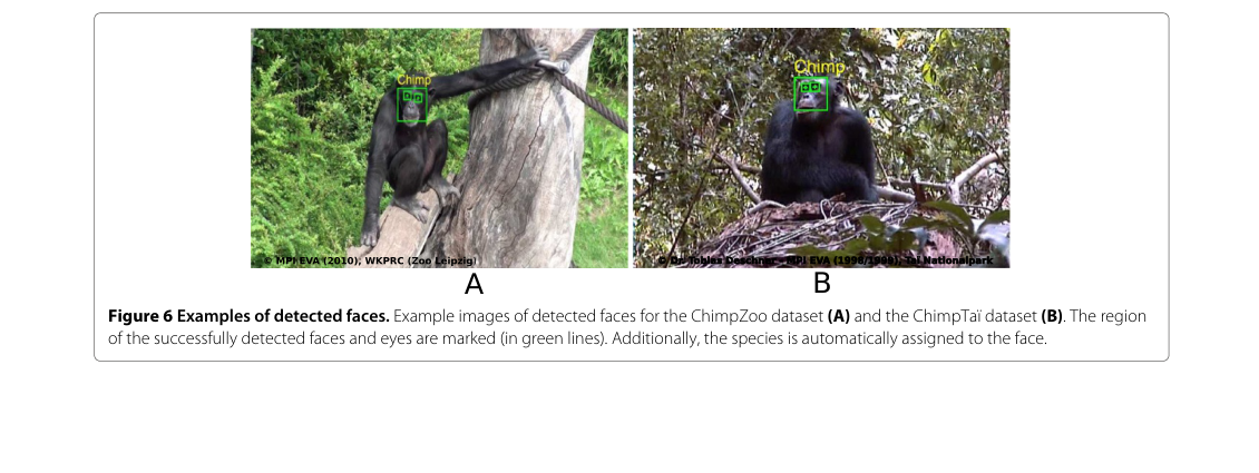
Understanding how primates move, communicate, and interact in their natural environments is one of the problems I care about most in biology. Since around 2011, researchers have built systems that detect primate faces, reconstruct 3D body pose from dozens of synchronized cameras, classify complex social behaviors, decode vocalizations, and generate realistic 3D avatars. The work now spans 14 topic areas, dozens of species from lemurs to great apes, and methods ranging from detection and pose estimation to facial action coding, hand tracking, species identification, and reinforcement learning.
Among the earliest automated chimpanzee face detection systems, with detected faces and eyes marked in green across zoo and field datasets. From Loos & Ernst, EURASIP J. Image Video Process. 2013, CC-BY 2.0.
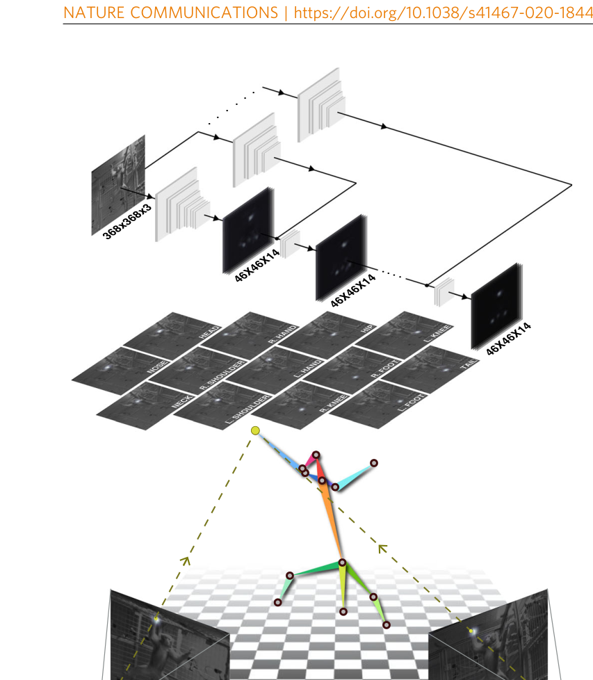
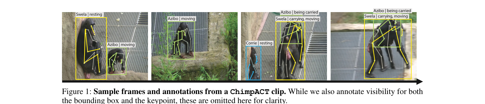
OpenMonkeyStudio reconstructs 13 body landmarks in 3D from 62 synchronized cameras, enabling markerless motion capture in freely moving macaques. From Bala et al., Nat. Commun. 2020, CC-BY 4.0.ChimpACT provides 160,500 annotated frames for joint detection, tracking, pose estimation, and behavior recognition in chimpanzees. From Ma et al., NeurIPS 2023.
But the diversity of approaches also shows how far we have to go. No single method, dataset, or species captures the full complexity of primate behavior — and too many models and datasets stay siloed or invisible to researchers working on related problems. That is why resources like this matter: connecting work across species, modalities, and methods so we can see where the gaps are and where open tools already exist. If you work at this intersection — or want to — we would love your contributions. Add a paper, open-source a model, share a dataset. Solving behavior understanding in primates is not something any one lab will crack alone; it will take a community building bridges across all of these approaches, and I believe this generation of researchers is up for it.
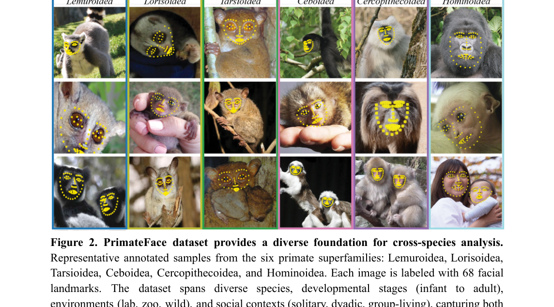
PrimateFace provides 260K+ annotated face images with 68 facial landmarks across six primate superfamilies, from lemurs to humans. From Parodi et al., bioRxiv 2025, CC-BY 4.0.]]>Felipe Parodi